Understanding the Least-Squares Method From the Perspectives of Calculus and Linear Algebra

The content below was generated entirely by machine translation. Please verify its accuracy. If anything is unclear, consult the Chinese source version.

I previously used the least-squares method when trying to implement some computer graphics papers, but at that time I understood it from the perspective of calculus. This year, after taking a linear algebra course, I found that it can also be explained using concepts from linear algebra and that this explanation is more intuitive (it provides a geometric understanding). Therefore, I plan to use this article to record two ways of understanding the least-squares method.

Before beginning, I first want to complain about the Chinese name of this method, “minimum two multiplication.” It just feels very strange: why is minimizing the square of the error called “two multiplication”? Well… after looking it up, I found that it was translated from Japanese, so I can only say that the quality of this translation is rather impressive… Although I really do not want to use this confusing name, there is nothing I can do because everyone uses it.

Definition of the Problem

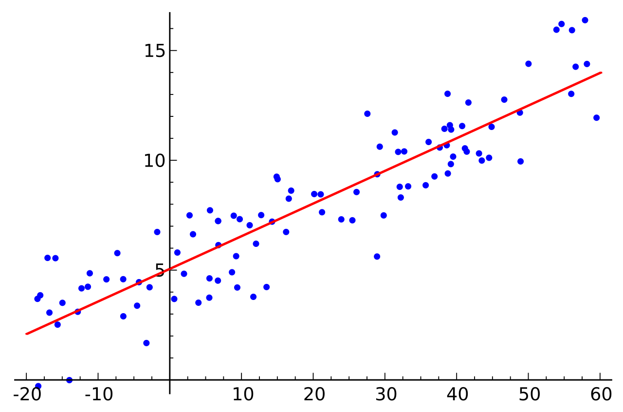
Before learning the least-squares method, we first need to understand what problem this algorithm is trying to solve. The most common use of the least-squares method is fitting data with a function and then using that function to predict the trend of the data. To fit data, we need to use a mathematical method to define what constitutes a good fit, and then try to make a function fit the data better.

Here, suppose there are $m$ data points $(x_i, y_i) \ \ i \in \{0, 1, \cdots, m\}$ . There is also a function $f(x)$ used to fit these data points. We define the error of an individual point as:

$s_i = f(x_i) - y_i$

Note that the meaning of the function $f(x_i)$ here is using $x_i$ to predict $y_i$ . You can understand these two values as scalars, but the least-squares method can actually also be used to fit vectors, because the formulas are exactly the same in both cases. For simplicity, we assume here that they are scalars.

Then the sum of squared errors is:

$I = \sum_{i=0}^m s_i^2 = \sum_{i=0}^m (f(x_i) - y_i)^2$

We want to adjust the parameters of this function to minimize this value.

Specifically, the function $f(x)$ can be expressed in the following form:

$f(x) = a_0\varphi_0(x) + a_1\varphi_1(x) + \cdots + a_n\varphi_n(x)$

Here, $a_i$ are the parameters that we need to adjust, while $\varphi_i(x)$ are some linearly independent functions.

Calculus Perspective

The content of this section mainly comes from this video. Its content is quite complete, but some parts move quickly and contain writing mistakes. I also watched it several times before understanding it.

We can express the error in the following form and then minimize this error from the perspective of calculus.

$\begin{align*} I(a_0, \cdots, a_n) &= \sum_{i=0}^m w(x_i) (f(x_i) - y_i)^2 \\ I(a_0, \cdots, a_n) &= \sum_{i=0}^m w(x_i)\left(\sum_{j=0}^n [a_j\varphi_j(x_i)] - y_i\right)^2 \end{align*}$

Writing it in this form expresses our objective more clearly: minimizing the error by adjusting the parameters $a_0, \cdots, a_n$ .

Note that, when summing the squared error of each data point, an additional weight $w(x_i)$ appears here. This weight makes it more convenient to adjust the importance of each data point.

From calculus, we know that the derivative of a function must be 0 when the function reaches an extremum. We can use this property to adjust the parameters from the perspective of calculus so that the error is minimized. However, this extremum may be either a minimum or a maximum. When calculating the error $I$ , only one minimum can exist (you can imagine the situation in which all parameters are set to $\infty$ ).

Because $I$ is a multivariable function, we need to use partial derivatives to find the minimum with the method above:

$\frac{\partial I}{\partial a_k} = 2\sum_{i=0}^m w(x_i)\left(\sum_{j=0}^n[ a_j\varphi_j(x_i)] - f(x_i)\right)\varphi_k(x_i) = 0 \\$

In the partial derivative above, everything other than $a_k$ can be treated as a constant. This is because the definition of a partial derivative is the effect on the error $I$ caused by changing the parameter $a_k$ .

When $\frac{\partial I}{\partial a_k} = 0$ , we can say that, when only the parameter $a_k$ is adjusted, the error has already reached its minimum. However, because every parameter can be adjusted, we want $\frac{\partial I}{\partial a_k} = 0$ for every $k \in \{0, \cdots, n\}$ .

In this way, we obtain a system of linear equations. When seeing a system of linear equations, the first thought is certainly to represent it using linear algebra, which can greatly increase the solution speed.

After some transformations, we obtain the following formula:

$\begin{align*} 0 &= 2\sum_{i=0}^m w(x_i)\left(\sum_{j=0}^n[ a_j\varphi_j(x_i)] - f(x_i)\right)\varphi_k(x_i)\\ &= 2\sum_{i=0}^m\left(w(x_i)\varphi_k(x_i)\sum_{j=0}^n\left[a_j\varphi_j(x_i)\right] - w(x_i)y_i\varphi_k(x_i) \right) \\ &= \sum_{i=0}^m\left(w(x_i)\varphi_k(x_i)\sum_{j=0}^n\left[a_j\varphi_j(x_i)\right]\right) - \sum_{i=0}^m\left[w(x_i)y_i\varphi_k(x_i)\right] \end{align*}$

Because we want to move toward a linear-algebra representation, we can express the following summation as a dot product:

$\sum_{i=0}^m\left[w(x_i)y_i\varphi_k(x_i)\right] \\ = \vec{w} \cdot \vec{y} \cdot \vec{\varphi_k}$

Here, $\vec{w} = w(x_i) \ i \in \{0, \cdots, m\}$ , $\vec{y} = y_i \ i \in \{0, \cdots, m\}$ , and $\vec{\varphi_k} = \varphi_k(x_i) \ i \in \{0, \cdots, m\}$ .

Similarly, the other part of the expression can also be represented as a dot product:

$\sum_{i=0}^m\left(w(x_i)\varphi_k(x_i)\sum_{j=0}^n\left[a_j\varphi_j(x_i)\right]\right) \\ = \vec{w} \cdot \vec{\varphi_k} \cdot \sum_{j=0}^n \vec{a_j} \cdot \vec{\varphi_j} \\ = \sum_{j=0}^n \vec{w} \cdot \vec{\varphi_k} \cdot \vec{\varphi_j} \cdot \vec{a_j}$

Then, if:

$\vec w \cdot \vec y \cdot \vec \varphi_k = \sum_{j=0}^n \vec{w} \cdot \vec{\varphi_k} \cdot \vec{\varphi_j} \cdot \vec{a_j}$

the partial derivative of the error is 0; that is, $\frac{\partial I}{\partial a_k} = 0$ .

Of course, our final goal is to write this expression as a matrix-multiplication equation to increase the solution speed. Looking carefully at the right-hand side of the equation, we can actually see that this summation is essentially also a dot product.

$\sum_{j=0}^n {\color{red}\vec{w} \cdot \vec{\varphi_k} \cdot \vec{\varphi_j}} \cdot \vec{a_j}$

To make this easier to understand, denote the part marked in red as $\vec A_k = [\vec{w} \cdot \vec{\varphi_k} \cdot \vec{\varphi_0}, \cdots, \vec{w} \cdot \vec{\varphi_k} \cdot \vec{\varphi_n}]$ . It is an $n$ -dimensional vector, so this summation is $\vec A_k \cdot \vec a$ , where $a = [a_0, \cdots, a_n]$ .

Similarly, we can denote $\vec w \cdot \vec y \cdot \vec \varphi_k$ as $B_k$ (a scalar).

Thus, solving the following system of equations solves the least-squares problem:

$\begin{cases} \vec A_0 \cdot \vec a = B_0 \\ \vec A_1 \cdot \vec a = B_1 \\ \qquad \vdots \\ \vec A_m \cdot \vec a = B_m \end{cases}$

This form is very familiar and can be represented directly in matrix form.

$\begin{bmatrix} A_{00} & A_{01} & \cdots & A_{0n} \\ A_{10} & A_{11} & \cdots & A_{1n} \\ \vdots & & \ddots & \\ A_{m0} & A_{m1} & \cdots & A_{mn} \\ \end{bmatrix} \cdot \begin{bmatrix} a_0 \\ a_1 \\ \vdots \\ a_n \\ \end{bmatrix} = \begin{bmatrix} B_0 \\ B_1 \\ \vdots \\ B_m \\ \end{bmatrix}$