The content below was generated entirely by machine translation. Please verify its accuracy. If anything is unclear, consult the Chinese source version.

~~Recently~~ (it has been a week since I finished RTOW, and I am only writing these notes now—truly lazy) I spent some time finishing Ray Tracing in One Weekend (hereafter RTOW) ~~I really am not good enough; I did not finish this thing in one weekend~~ and also wrote the code.

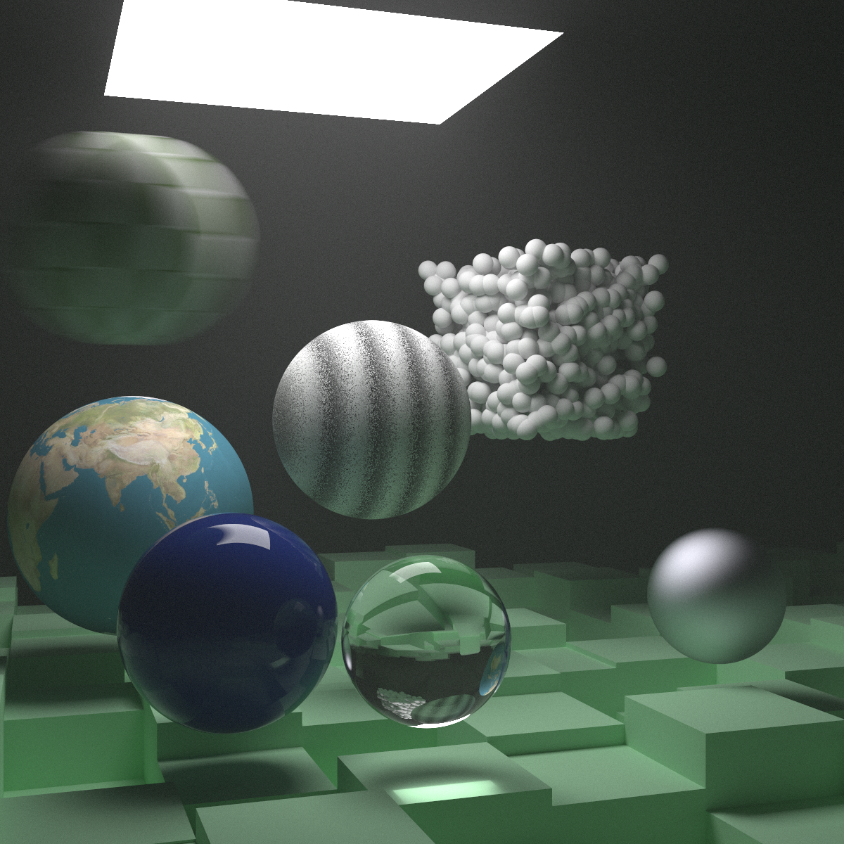
The book is excellent, and the final rendering was beyond my expectations (the cover image). However, I previously knew nothing about computer graphics, so many basic concepts were unfamiliar. The book sometimes passes over basic knowledge, mathematical derivations, and proofs, so I am writing down my own thought process here.

Implementing a Lambertian Material

The book creates a Lambertian diffuse material as follows:

class lambertian : public material {
   public:
    lambertian(const color& alb) : albedo(alb) {}
    virtual optional<pair<ray, color>> 
    get_ray_out(const ray& r_in, const hit_rec& rec) const override {
        vec3 ref_dir = rec.norm + rand_unit_vec(); // Note this line.
        if(ref_dir.near_zero()) // If rand_unit_vec() equals -rec.norm.
            ref_dir = rec.norm;
        ray ref_ray(rec.hit_pt, ref_dir);
        return make_pair(ref_ray, albedo);    
    }
    color albedo;  // Albedo.
};

After a ray hits a diffuse material, the scattered ray starts at the hit point (rec.hit_pt) and its direction is a random unit vector plus the normal at the hit point.

Why add the normal? Why not simply choose a random vector in a hemisphere?

Radiometry

To answer this, we need some knowledge of radiometry. In ray tracing we care about the light received by a camera (or the human eye), so the explanation below uses the camera’s perspective.

Basic Units

We first need to consider exactly which physical quantity a camera sensor receives. Clearly, it receives energy—or, in other words, a number of photons arriving at the sensor. We therefore regard the physical quantity received by the sensor as radiant energy, denoted by $Q$ and measured in joules.

Energy alone, however, does not represent an object’s brightness very well. After all, photographing the same scene with an exposure of one minute and an exposure of $\frac{1}{100}$ second will certainly produce different results.

Although the sensor ultimately receives energy, we can continue obtaining more energy simply by exposing, or integrating, for a longer time while holding the camera.

Naturally, this suggests dividing the received energy by the time spent collecting it. This gives the unit known as radiant flux:

$\Phi = \frac{\mathrm{d}Q}{\mathrm{d}t}$

That is, radiant flux is the energy the sensor can receive per unit time.

Conversely, it can also describe the energy transmitted by a light source per unit time.

This still cannot completely describe an object’s brightness. If we use a larger sensor in the camera, the larger sensor can receive more energy per unit time.

Using a larger sensor while observing something cannot change the brightness of the object itself. We must therefore divide the received radiant flux by area, obtaining radiant flux per unit area. This unit is called irradiance.

For a light source, using a larger emitting surface can likewise provide more total radiant flux, while the flux provided per unit area remains unchanged.

$E = \frac{\rm{d}\Phi}{\rm{d}A}$

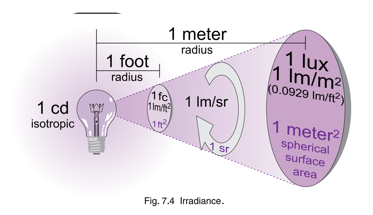
We find that as the viewing distance increases, a larger area is required to collect the same luminous flux, so irradiance becomes smaller. This plainly conflicts with common experience: as distance increases, the brightness we observe does not decrease significantly. When attenuation does occur, it is mainly because light encounters many tiny particles while propagating.

What is happening? Intuitively, although a more distant observer receives less radiant flux, the object also appears smaller to the human eye.

For example, consider a lamp with a very large area and another lamp with a very small area. If they emit the same radiant flux, the smaller lamp is clearly brighter.

Thus, the flux received directly by the eye decreases, but the observed area of the object decreases correspondingly. These two changes cancel, leaving the observed brightness unchanged. We therefore need a physical quantity that describes the apparent size of the object seen by the eye. Dividing irradiance by this quantity will then genuinely describe brightness. That quantity is the solid angle.

We can imagine the eye’s field of view as a sphere whose center is the eye. Every point on the sphere is consequently the same distance from the eye. If many equally sized objects are placed on the surface of this sphere, they are the same distance from the eye and therefore appear to have the same size.

Objects at different distances can all be projected onto this sphere. An object whose projection occupies a larger area on the sphere appears larger to the eye.

From the perspective of a light source, we sometimes want to focus on the source’s effect in a particular direction—how much it illuminates that direction and how much radiant flux it provides. A solid angle can also be introduced for that analysis.

The solid angle is therefore defined as the projected area of an object on a unit sphere, whose radius is 1.

It is calculated as follows and measured in steradians (sr):

$\Omega = \frac{a}{R^2}$

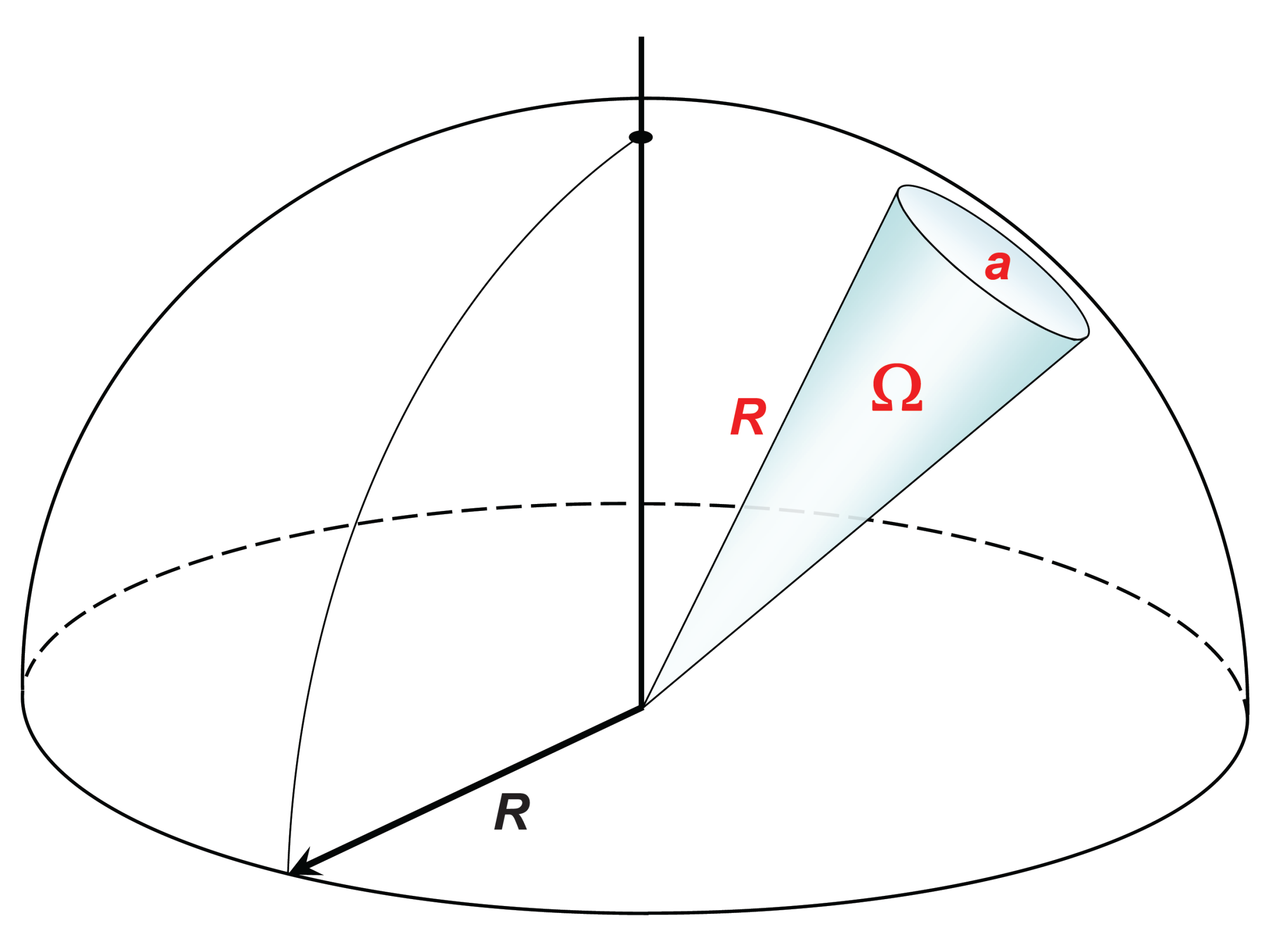
Here, $a$ is the area projected onto a sphere, which need not be a unit sphere, and $R$ is the sphere’s radius.

With the solid angle, we can genuinely describe the apparent size of the object seen by the eye. Modifying irradiance further gives the physical quantity called radiance:

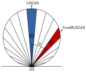
$L_\theta = \frac{\rm{d} \Phi}{\rm{d}A\cos(\theta)\rm{d}\Omega}$

In this formula, $A$ is the area of the photosensitive surface element, and $\Omega$ is the solid angle. The factor $\cos(\theta)$ calculates the area of an object parallel to the spherical surface, as shown below:

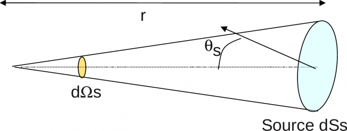
Here, $\theta$ is the angle between the object’s surface normal and the sphere’s normal. When $\theta$ is $0$ , $\rm{d}A\cos(\theta)$ is largest. When $\theta$ is $\frac{\pi}{2}$ , the object’s surface is perpendicular to the spherical surface, so rays emitted from the sphere do not intersect the object at all, and $\rm{d}A\cos(\theta)$ is 0.

Radiance already describes the brightness characteristics of most objects quite perfectly. The preceding discussion, however, concerns area light sources or sensors with a nonzero area. A point light has no area, so radiance is meaningless for it because the formula divides by area.

At other times, we may not care about the areas of the light source and sensor and may simply want to know the radiant flux emitted or received in a direction. We then need another physical quantity—radiant intensity—which is obtained by removing the division by area from radiance:

$I = \frac{\rm{d}\Phi}{\rm{d}\Omega}$

Lambert’s Cosine Law

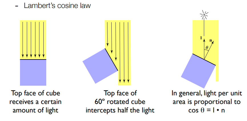
Mathematically:

$I_\theta=I_n\times\cos\theta,$

where $I_n$ is the intensity when the surface normal is parallel to the ray. The larger the angle between the observer’s normal and the ray, the less flux is received. The cosine computes the area of the surface projected onto a plane perpendicular to the ray.

Lambertian Materials and Diffuse Reflection

Wikipedia describes a Lambertian radiator as a source whose spatial intensity distribution follows the cosine law; its intensity decreases with angle. A Lambertian surface, however, has the same radiance from every viewing direction.

The definitions explain why these statements are consistent:

$L_\theta=\frac{\mathrm d\Phi}{\mathrm dA\cos\theta\mathrm d\Omega},\qquad I_\theta=\frac{\mathrm d\Phi}{\mathrm d\Omega}\cos\theta.$

Thus the cosine cancels between numerator and denominator for radiance. Intensity depends on angle, but radiance does not. From the observer’s viewpoint, an oblique surface also appears smaller, which cancels the reduced flux.

Why Is the Code Written This Way?

Ray tracing follows rays backwards, from the camera toward the light. A camera point $B$ may receive contributions from many rays leaving an object point $A$ , so after tracing from $A$ to $B$ we must choose the next direction.

I understand this as tracing radiant intensity: each pixel has the same area, so its color depends on flux from a direction. Lambert’s cosine law must therefore be considered when measuring the contribution to $B$ .

The book samples each pixel repeatedly:

……
color pixel_color(0, 0, 0);
for (int s = 0; s < samples_per_pixel; ++s) {
    auto u = (i + random_double()) / (image_width-1);
    auto v = (j + random_double()) / (image_height-1);
    ray r = cam.get_ray(u, v);
    pixel_color += ray_color(r, world);
}
write_color(std::cout, pixel_color, samples_per_pixel);
……

There are two ways to model the cosine attenuation. Choose a random direction on the unit hemisphere and multiply by the cosine of its angle with the normal:

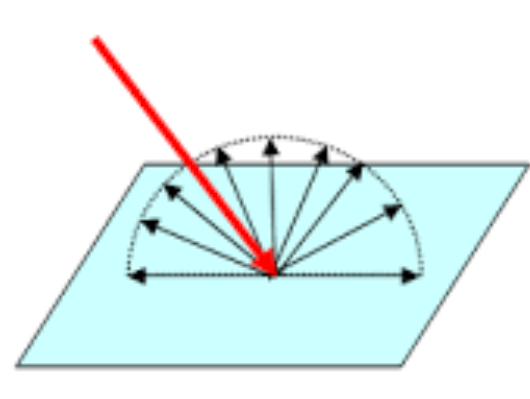
Or use $\cos\theta$ as the probability density function for choosing directions, eliminating the explicit attenuation:

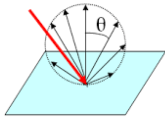
The book chooses the second method. If $\cos\theta$ is treated as the length of a segment making angle $\theta$ with the normal and one endpoint is fixed at $B$ , the result is a circle tangent to $B$ (a sphere in three dimensions):

I do not currently know how to prove this, but it is correct. RTOW uses it by adding the hit-point normal to a random unit vector:

1	vec3 ref_dir = rec.norm + rand_unit_vec();

One remaining question is why the light received at $B$ is uniformly scattered around it. We are tracing radiant intensity, so should we calculate the angle between the surface normal and the camera and apply cosine attenuation?

As the angle increases, the surface area corresponding to one pixel also increases, cancelling the cosine attenuation. Since each sample chooses an arbitrary position inside the pixel, repeated samples cover the surface corresponding to that pixel. If we explicitly applied cosine attenuation, we would likewise take more samples from regions with larger angles, because those regions cover a larger area.

References: