The content below was generated entirely by machine translation. Please verify its accuracy. If anything is unclear, consult the Chinese source version.

Implementing the Camera Class

In addition to the Lambertian material, another interesting part of RTOW is the implementation of the camera class, especially the depth-of-field portion.

Positioning the Camera

Let us first look at a relatively simple part of the camera class—the camera’s position. Three parameters are enough to determine the camera’s position: the position of the camera itself (lookfrom), the position at which the camera is taking a photograph (lookat), and a vector representing the position above the camera (vup). The figure in the book explains this very well:

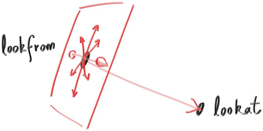
In the constructor, we need to convert these three parameters into three parameters representing the camera’s orientation, and also handle the focal length, aperture, and FOV. The book does not spend much space on this part. It took me quite a while to understand it, so below are some thoughts about the implementation in the book.

Because I made some small changes to the code in the book (mainly naming?), I will first paste the code:

#pragma once
#include "rtow.h"

// f8 here is double (a float occupying eight bytes).
class camera {
   public:
    camera(vec3 lookfrom, vec3 lookat, vec3 vup = vec3(0, 1, 0), f8 vfov = 90,
           f8 asp_ratio = 16.0 / 9.0, f8 aperture = 0, f8 foc_len = 1) {
        f8 deg_fov = deg2rad(vfov);
        f8 half_hei = tan(deg_fov / 2);  // Opposite side divided by adjacent side, while the adjacent side is 1.
        f8 half_wid = half_hei * asp_ratio;

        cam_z = (lookfrom - lookat).unit_vec();
        // z points opposite to the direction in which the lens is pointing.
        cam_x = cross(vup, cam_z).unit_vec();  // Perpendicular to both vup and z.
        cam_y = vup.unit_vec();

        horizon = 2 * half_wid * cam_x * foc_len; // The horizontal and vertical frame vectors on the focal plane.
        vertic = 2 * half_hei * cam_y * foc_len;

        orig = lookfrom;

        lower_left_corner = orig - horizon / 2 - vertic / 2 - cam_z * foc_len; // The lower-left corner of the focal plane.

        len_radius = aperture / 2;
    }

    inline ray get_ray(f8 x, f8 y) const {
        // The ranges of x and y are [0, 1].
        // Coordinates of the pixel on the camera sensor.
        vec3 rd = len_radius * rand_unit_disk();
        vec3 offset = cam_x * rd.x() + cam_y * rd.y(); 

        ray r;
        r.orig = orig + offset;
        r.dir = lower_left_corner + x * horizon + y * vertic -
                orig - offset;  
            // Produce a vector from orig + offset to the corresponding pixel.
            // This is because a ray is represented by orig + t * dir.
        return r;
    }

    vec3 orig;               // Camera position.
    vec3 lower_left_corner;  // Lower-left corner of the image.
    vec3 horizon, vertic;    // Image dimensions (or the size of the plane at distance foc_len from the camera).
    vec3 cam_x, cam_y, cam_z;// Camera orientation.
    f8 len_radius;           // Aperture radius.
};

The following figure describes the relationships among the variables in the code:

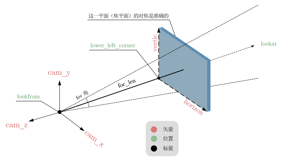
It is relatively easy to understand the code using this figure.

The following code first calculates two variables, half_hei and half_wid:

1
2
3

f8 deg_fov = deg2rad(vfov);
f8 half_hei = tan(deg_fov / 2);  // Opposite side divided by adjacent side, while the adjacent side is 1.
f8 half_wid = half_hei * asp_ratio;

They represent the size of the image seen at a distance of one unit in front of the camera. Next, the three vectors cam_x, cam_y, and cam_z need to be calculated as follows:

cam_z = (lookfrom - lookat).unit_vec();
// z points opposite to the direction in which the lens is pointing.
cam_x = cross(vup, cam_z).unit_vec();  // Perpendicular to both vup and z.
cam_y = vup.unit_vec();

cam_z represents a direction from lookat to loofrom, which is opposite to the position at which the camera is actually taking the photograph.
The calculation of cam_x uses the cross product of vectors. In three-dimensional space, if $u = v \times w$ , then $u$ is perpendicular to both $v$ and $w$ . Of course, there are two vectors satisfying this condition, and the right-hand rule can be used to determine which one. From the preceding definition, we can conclude that cam_x is perpendicular to both cam_z and vup (that is, cam_z).
cam_y is the unit vector of vup.

Although I roughly understood the geometric meaning of the cross product of three-dimensional vectors, I did not previously completely understand how it was derived. I found the explanation in the following blog particularly clear; even I, a beginner, could understand it:

https://www.cnblogs.com/qilinzi/archive/2013/05/09/3068158.html

The calculations of horizon, vertic, and lower_left_corner are relatively simple, so I will not explain them here; they are all marked in the figure.

Implementing Depth of Field

Depth of Field in Reality

To understand how a computer simulates depth of field, we first need a basic understanding of the structure of a camera lens, as follows:

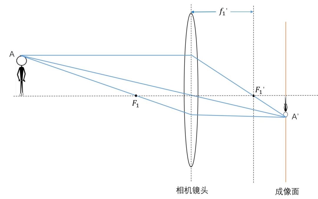
Without a lens, light originating from point A can propagate in many directions, and each direction reaches a different position on the imaging plane. In the end, the color of each point on the imaging plane is contributed by many different rays, naturally producing a blurry image.

After adding a lens and considering point A again, we can observe that the rays originating from point A in every direction eventually converge at one specific point on the imaging plane, namely A’. The resulting image is clear.

More generally, a lens satisfies the following two conditions:

Rays emitted in different directions from the same point must converge at the same point after passing through the lens.
Rays emitted from different points on the same plane converge at different points after passing through the lens.

There is one prerequisite: the point must be on the focal plane of the camera. If the distance between a point and the camera’s imaging plane is not the focal length, the following occurs:

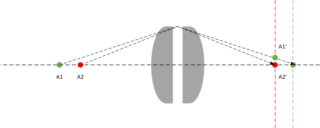
If the imaging plane is the green one, A1 is on the correct focal plane. If the imaging plane is the red one, A2 is on the correct focal plane.

For convenience, let us analyze A1. On the red imaging plane, we find that rays originating in two directions (horizontally and diagonally) converge at different points. On the green imaging plane, they converge at only one point.

Although they converge at different points, the degree of difference varies. Imagine moving A1 further to the left. Then the position of A1’ on the red imaging plane must become higher. Conversely, if A1 is moved to the right, the position of A1’ on the red imaging plane also falls, eventually converging at the correct point. If it continues moving right, the position of A1’ on the red imaging plane continues to fall. Eventually, the distance on the imaging plane between the rays originating horizontally and diagonally from A1 increases.

Alternatively, if we increase the size of the lens, more rays originating from A1 at different angles can enter the lens and then reach the imaging plane. In this case, the position of A1’ on the red imaging plane becomes higher. We can imagine that the lens has been pulled upward, and the triangle formed by the rays has also been pulled upward (I was too lazy to draw the figure myself, so I used an image from the Internet to explain it this way).

From the preceding figure, we can see that, theoretically, there is only one distance at which the camera can produce a sharp image; slightly more or less is no longer sharp. In reality, however, the resolving ability of the human eye is not that strong. The range of distances that can produce a sharp image when the camera takes a picture (that the human eye considers sharp) is called the depth of field, as follows:

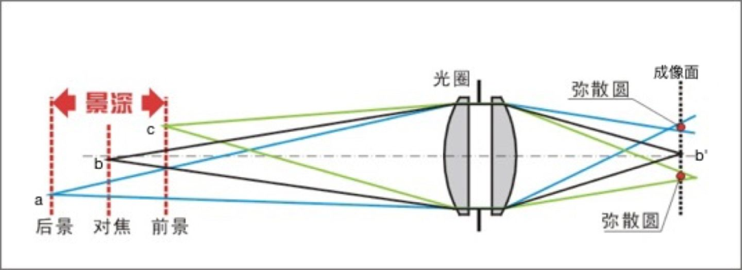
We can think about the influence of the lens size, or radius, mentioned above from the perspective of depth of field. In reality, the radius of the lens does not change. The usual method is to add an adjustable “gate” to the lens—the aperture—to control the light entering the lens, as follows:

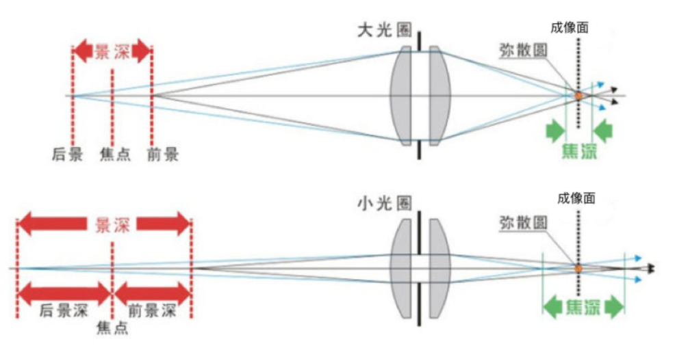
We can see that a larger aperture reduces the depth of field, and vice versa.

Actual Implementation

Earlier, we considered that rays originating from one point at different directions converge at different points on the imaging plane when the focal length is incorrect. During actual rendering, however, we consider the contributions of different rays to a particular pixel on the imaging plane.

Therefore, when the aperture is large, more rays from different directions should simultaneously contribute to one point on the imaging plane, producing a blur. See the figure below, which shows the implementation of depth of field in RTOW:

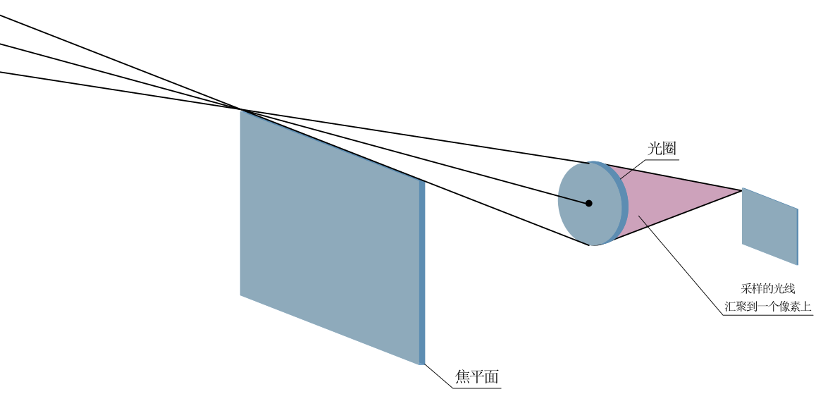
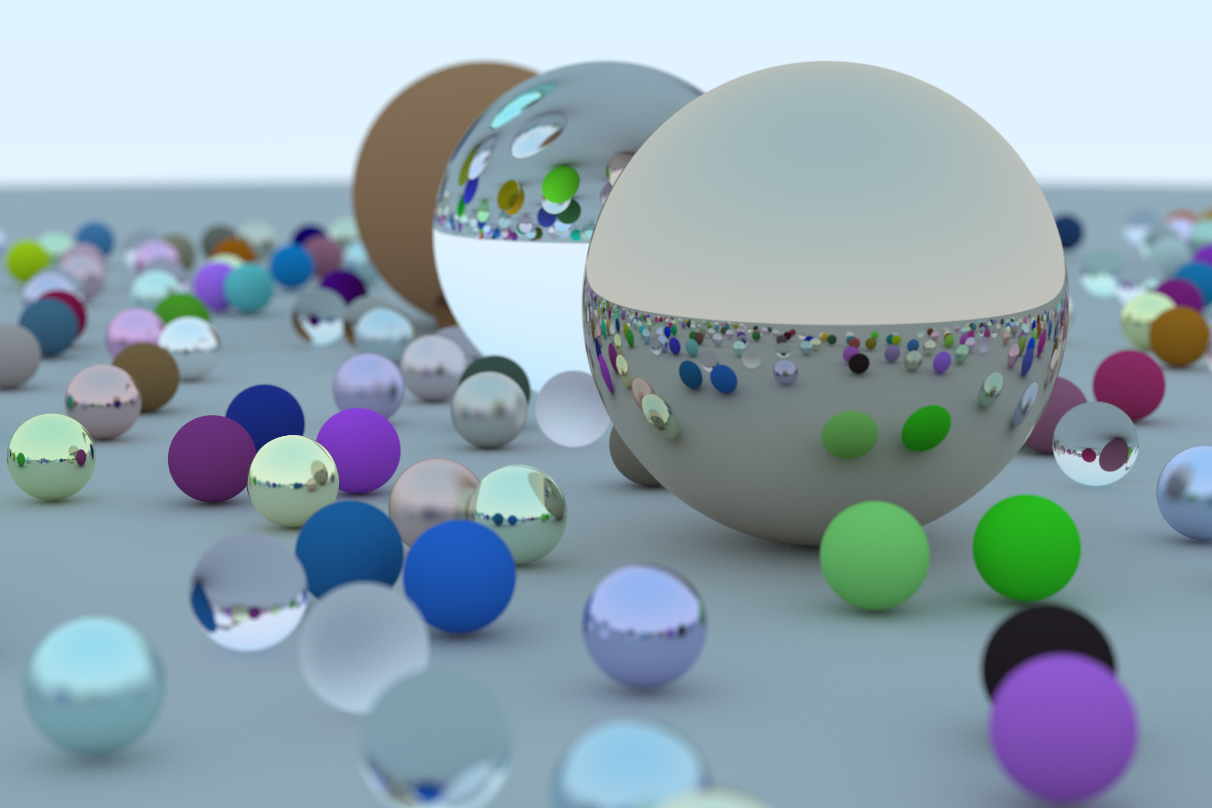
In the code, we randomly select a point on the aperture and then trace a ray from the aperture to the corresponding pixel on the focal plane. Finally, we average the contributions of the sampled rays. The larger the aperture, the smaller the depth of field. Moreover, because every ray must pass through the corresponding point on the focal plane, we can ensure that the focal plane is always sharp.

Compared with how a real lens works, this is quite different, but it achieves the same effect. This is also due to the characteristics of ray tracing: it traces “backward” starting from the pixel. Therefore, we do not focus on the issue of rays emitted by one point in a real lens converging at different positions on the imaging plane. Instead, we think from another angle: how many rays emitted by different points affect one pixel. I have to say that this implementation in the book is really impressive.

References: