The content below was generated entirely by machine translation. Please verify its accuracy. If anything is unclear, consult the Chinese source version.

After more than a month of intermittent work, I finally finished the material in the second book. As with the previous two articles, this article records some parts that personally took me a relatively long time to understand, as well as some new features I added on top of the original book.

For features already present in the original book, I use the book’s code directly; for features I added, I use my own code. Because my code differs substantially from the original book—even for features that were already there—a single code excerpt may be hard to understand. You can refer to my GitHub repository here: https://github.com/ttzytt/RTOW

`bvh_node`

This section is mainly about a few small details that I did not fully understand at the time. First is this:

bvh_node::bvh_node(
    std::vector<shared_ptr<hittable>>& src_objects,
    size_t start, size_t end, double time0, double time1
)

The first issue is the range handled by this constructor. Each subtree is not responsible for the hittable at position end. In other words, this constructor handles an interval of the form [start, end).

This also explains how sort is used in the code:

1	std::sort(objects.begin() + start, objects.begin() + end, comparator);

The interval actually sorted by std::sort() is of the form [) (~~I somehow never noticed this before~~). Therefore, objects.begin() + end does not include end here.

When sorting containers such as a vector, the usual method is sort(vec.begin(), vec.end()). At first glance, this appears not to include the element at .end(), but .end() actually points to an empty position—or, put another way, the position after the last element (~~I had not noticed this before either~~). Consequently, this form sorts the entire vector.

Spherical Texture Coordinates

class sphere : public hittable {
    ...
    private:
        static void get_sphere_uv(const point3& p, double& u, double& v) {
            // p: a given point on the sphere of radius one, centered at the origin.
            // u: returned value [0,1] of angle around the Y axis from X=-1.
            // v: returned value [0,1] of angle from Y=-1 to Y=+1.
            //     <1 0 0> yields <0.50 0.50>       <-1  0  0> yields <0.00 0.50>
            //     <0 1 0> yields <0.50 1.00>       < 0 -1  0> yields <0.50 0.00>
            //     <0 0 1> yields <0.25 0.50>       < 0  0 -1> yields <0.75 0.50>

            auto theta = acos(-p.y());
            auto phi = atan2(-p.z(), p.x()) + pi;

            u = phi / (2*pi);
            v = theta / pi;
        }
};

This code uses the atan2 function rather than the ordinary atan function. We know that the trigonometric function tan returns the slope of the tangent for the corresponding angle on a circle. Accordingly, atan returns the angle corresponding to a slope. When calculating texture coordinates, however, what we actually want is to obtain the corresponding angle from a coordinate on the circle. Of course, we could directly use atan(y/x), first calculating the slope and then the angle.

The problem is that a circle is described by an equation rather than a function: one x-coordinate can correspond to multiple y-coordinates. A single slope can therefore correspond to multiple angles. More specifically, although $(x, y)$ and $(-x, -y)$ correspond to different angles, their slopes are identical. If we used atan, we would also have to check the signs of the coordinates ourselves; atan2 effectively performs this work for us.

Checkerboard Texture

Implementation in the Book

virtual color value(double u, double v, const point3& p) const override {
    auto sines = sin(10*p.x())*sin(10*p.y())*sin(10*p.z());
    if (sines < 0)
        return odd->value(u, v, p);
    else
        return even->value(u, v, p);
}

This code multiplies together the values of the three components after multiplying them by $\pi$ . If the result is positive, it returns one color; otherwise, it returns the other. This may be difficult to understand at first glance, but it becomes much clearer if we first draw a two-dimensional version:

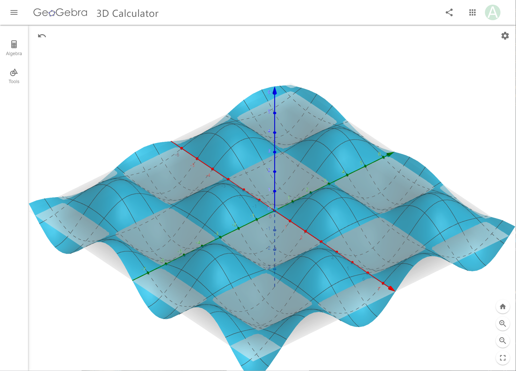
After adding another axis, the sign of $\sin()$ changes periodically, so we can see distinct layers. The colors flip between layers, while within a single layer the sign remains unchanged, so it can be treated directly as the two-dimensional version above:

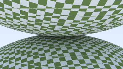
To be honest, however, trigonometric functions are not the only periodic functions. The book writes it this way only to obtain a positive or negative sign rather than a specific value, so using $\sin$ really wastes some computing resources.

One very simple example would be to take $x$ modulo $100$ : return a positive number if the result is less than $50$ , and a negative number otherwise. For a more concise form, it could also be written as follows:

$y=\operatorname{mod}\left(x,100\right)-50$

Checkerboard Only on the Surface

It is not difficult to see that the checkerboard in the book is based on a point’s absolute coordinates in space. That is why the layering shown above appears. Since we can already calculate texture coordinates on a sphere (the book also discusses texture coordinates for other hittable objects, such as rectangular patches), we can instead create a checkerboard texture based on the object’s surface, as follows:

class surface_checker : public texture {
   public:
    using text_array = std::vector<std::shared_ptr<texture>>;
    surface_checker() = default;
    surface_checker(const text_array& _texts,
            const std::pair<f8, f8> _siz = {514, 114})
        : texts(_texts), polar_azim_siz(_siz) {}

    virtual color value(f8 polar, f8 azim, const pt3& p) const override {
        int x_idx = (i8)(azim * polar_azim_siz.first);
        int y_idx = (i8)(polar * polar_azim_siz.second / 2.0); 
        // The polar angle spans only a hemisphere. To obtain polar_azim_siz.second
        // cells vertically over the whole sphere, divide by two first.
        return texts[(x_idx + y_idx) % texts.size()]->value(polar, azim, p);
    }

    text_array texts;
    std::pair<f8, f8> polar_azim_siz;  // Number of cells vertically and horizontally
};

Here, text_array allows the checkerboard to contain more than two colors, while (azim * polar_azim_siz.first) expands the original texture-coordinate range of $[0, 1]$ to polar_azim_siz.first, ensuring that the sphere has polar_azim_siz color changes. This produces the following result:

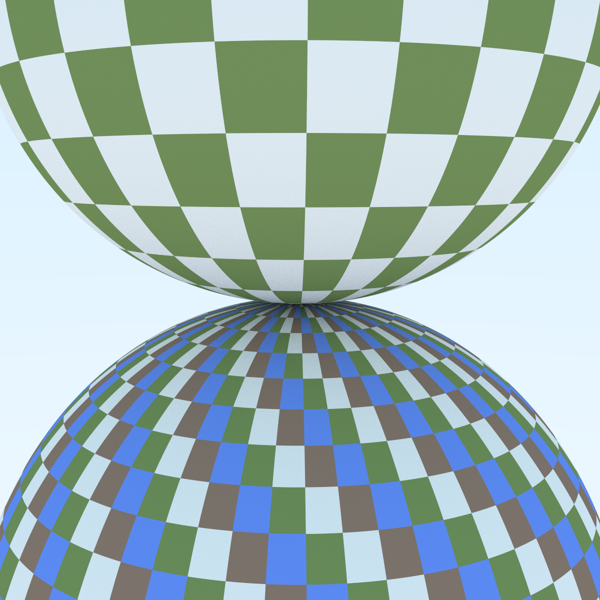
The code that generates this scene is as follows:

scene surf_check_sc() {
    hittable_list world;

    auto checker1 = make_shared<surface_checker>(
        surface_checker::text_array{
            make_shared<fixed_color>(color(0.2, 0.3, 0.1)),
            make_shared<fixed_color>(color(0.9, 0.9, 0.9)),
            make_shared<fixed_color>(color(0.3, 0.2, 0.15)),
            make_shared<fixed_color>(color(0.15, 0.3, 0.9))},
        std::pair<f8, f8>{60, 60});

    auto checker2 = make_shared<surface_checker>(
        surface_checker::text_array{
            make_shared<fixed_color>(color(0.2, 0.3, 0.1)),
            make_shared<fixed_color>(color(0.9, 0.9, 0.9)),
        },
        std::pair<f8, f8>{30, 30});

    world.add(make_shared<sphere>(pt3(0, -10, 0), 10,
                                  make_shared<lambertian>(checker1)));
    world.add(make_shared<sphere>(pt3(0, 10, 0), 10,
                                  make_shared<lambertian>(checker2)));

    f8 asp_ratio = 1.0;
    vec3 lookfrom = pt3(13, 2, 3) * 2;
    vec3 lookat = pt3(0, 0, 0);
    f8 vfov = 40.0;
    auto dist_to_focus = 10.0;
    auto aperture = 0;
    vec3 vup(0, 1, 0);
    auto cam_ptr = make_shared<camera>(lookfrom, lookat, vup, vfov, asp_ratio,
                                       aperture, dist_to_focus, aperture, 1.0);

    return scene(make_shared<bvh_node>(world), blue_sky_back_ptr, cam_ptr);
}

Perlin Noise

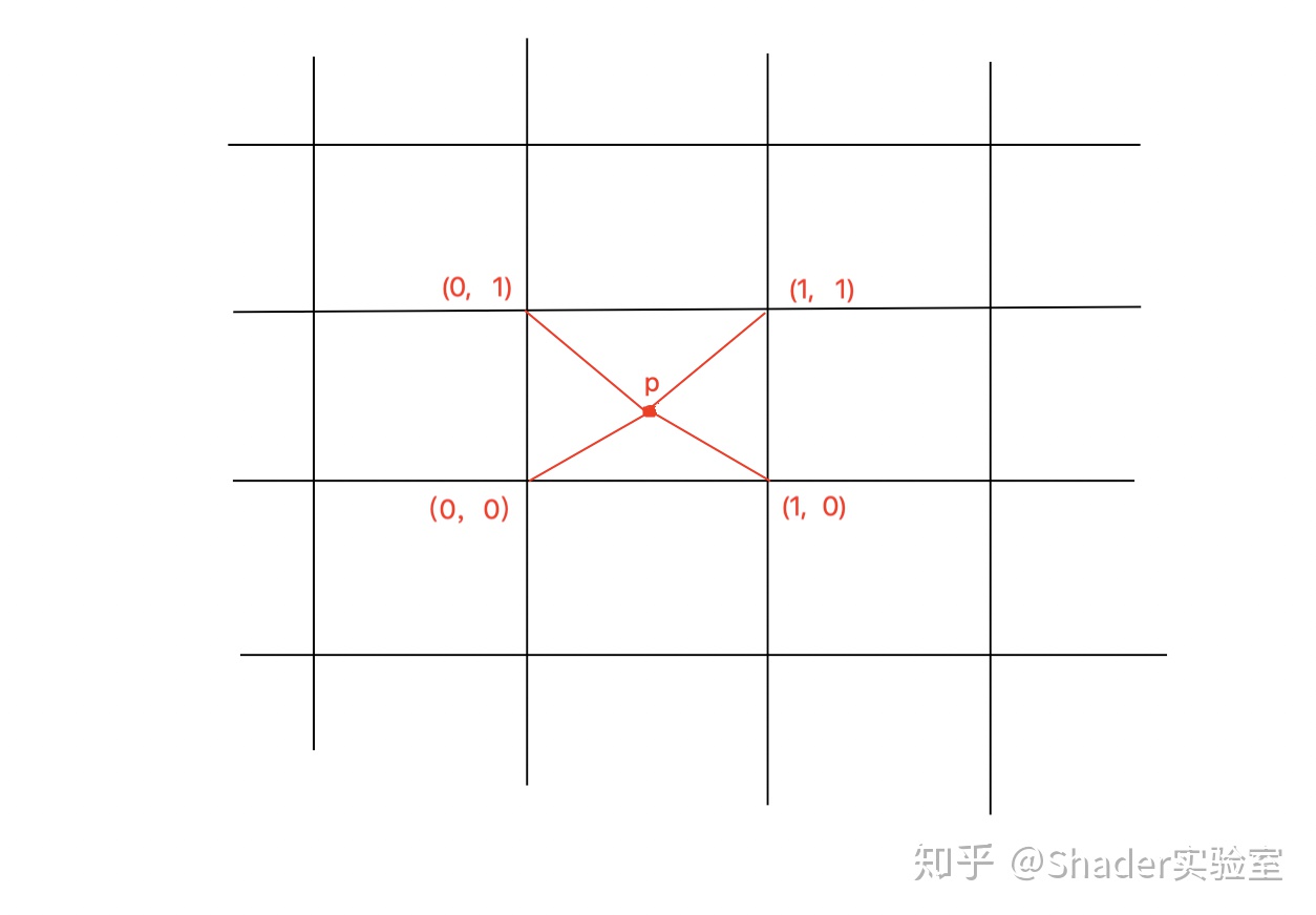
Perlin noise is one of the more difficult points in the book to understand, but Perlin noise is based on ordinary value noise. Value noise simply generates random numbers at integer coordinates in space and then uses those integer-coordinate values to linearly interpolate values at other coordinates (if you do not understand linear interpolation, see this link; I personally think it explains the idea very clearly).

It works roughly as follows

Random numbers are generated at the intersections of the vertical and horizontal lines—the integer coordinates. The value at point p in the figure is linearly interpolated from the four surrounding key points (that is, points with integer coordinates, which generate random numbers). Ultimately, the value at p depends on its distances from those four key points and the random values at the four points.

The following is an example of two-dimensional value noise:

The generating code is as follows:

import numpy as np
import matplotlib.pyplot as plt
from math import *

XLEN = 25 # Number of integer points to generate
YLEN = 25
DIFF = 0.05

ptsx = np.arange(0, XLEN, DIFF)
ptsy = np.arange(0, YLEN, DIFF)
xs, ys = np.meshgrid(ptsx, ptsy)
z_orig = np.random.random((XLEN + 1, YLEN + 1))
z_interped = np.zeros((round((XLEN) / DIFF), round(YLEN / DIFF)))

def lerp(a, b, t):
    return a + t * (b - a)

def lerp2(ld, rd, lu, ru, tx, ty): # Two-dimensional linear interpolation
    # left down, right down, left up, right up
    upmid = lerp(lu, ru, tx)
    dnmid = lerp(ld, rd, tx)
    return lerp(dnmid, upmid, ty)

for i in range(XLEN):
    for si in range(round(1 / DIFF)):  # step i
        for j in range(YLEN):
            for sj in range(round(1 / DIFF)):
                z_interped[i * round(1 / DIFF) + si][j * round(1 / DIFF) + sj] = lerp2(
                    z_orig[i][j], z_orig[i + 1][j], z_orig[i][j + 1],  z_orig[i + 1][j + 1], DIFF * si, DIFF * sj)


plt.imshow(z_interped, cmap=plt.cm.gray)
plt.savefig("./2d.png", dpi = 150, format = 'png')
plt.show()

It is easy to see that this noise looks unnatural; you can even vaguely make out the coordinate axes in the image. Although the entire image looks relatively random, close inspection shows that it is assembled from many small, square patches of color.

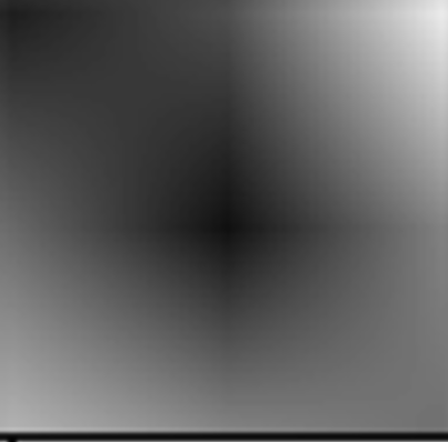
This happens because each key point has the same influence in every direction, while linear interpolation turns that influence into a diamond-like shape. The point in the center of the following image is a key point. Its random value is relatively low, so it is black, and we can see that the black region spreading outward from it has a diamond shape.

Changing this is also very simple: make a key point’s influence on its surroundings differ by direction. Since we need to represent a direction, vectors are a natural idea.

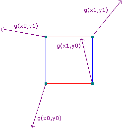
We now generate random unit vectors at each key point and denote them by $\vec{g_i}$ (the random vector generated at key point $i$ ), as follows

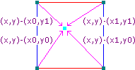
The question is now how to use these random vectors to produce different influences in different directions. One natural idea is to consider the position of a point relative to a key point. We can denote this displacement vector by $\vec{d_i}$ (the displacement from key point $i$ ), as shown below

If $\vec{d_i}$ and $\vec{g_i}$ point in similar directions, we can make the point brighter. Conversely, if $\vec{d_i}$ and $\vec{g_i}$ point in opposite directions, the point should be darker.

This effect can be achieved with a dot product, which is essentially the length obtained by projecting $\vec{d_i}$ onto $\vec{g_i}$ . The result is negative for opposite directions, positive for the same direction, and zero for perpendicular directions.

We record this dot product:

$\vec{v_i} = \vec{d_i} \cdot \vec{g_i}$

We can then linearly interpolate among the four surrounding points in the same way as value noise. In other words, we treat $\vec{v_i}$ as the value that used to reside at a key point in value noise. This value now changes for each position.

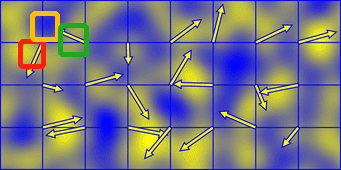
The following image demonstrates Perlin noise. Different arrows represent different $\vec{g_i}$ values; smaller values are bluer and larger values are yellower

Pay attention to the three boxes in the image.

Most of the red box is yellow because the displacement vectors of the points in this region have directions similar to the key point’s random vector.
Most of the yellow box is blue because the tail of the random vector at its lower-left key point points toward this region. In other words, the displacement vectors in this region are opposite to the random vector at that key point.
Most of the green box is yellow. Although this region lies in the direction opposite to the random vector of the key point on the left, linear interpolation is present and the region is closer to the random vector on the right, so it is influenced more strongly by the vector on the right.

It is very clear that the noise generated by Perlin noise does not have the blocky appearance of value noise.

Turbulence

Consider the following implementation of turbulence:

double turb(const point3& p, int depth=7) const {
    auto accum = 0.0;
    auto temp_p = p;
    auto weight = 1.0;

    for (int i = 0; i < depth; i++) {
        accum += weight*noise(temp_p);
        weight *= 0.5;
        temp_p *= 2;
    }

    return fabs(accum);
}

The turb function itself is relatively easy to understand: it superimposes Perlin noise at many frequencies using certain weights. The final fabs appears to keep the returned value within the $[0, 1]$ range, but it actually has another purpose. For example, if we replace the last line with return (accum + 1) * 0.5, the returned value also lies within the range, but the result looks very different from the original implementation.

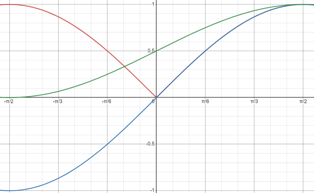
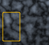
In the following figure, the blue line is the graph of $y = \sin x$ , the red line is the graph of $y = |\sin x|$ , and the green line is $y = \left(\sin\left(x\right)+1\right)\times 0.5$ :

With the green-line correction, regions that were originally dark remain dark afterward, and vice versa. With the red-line correction, only regions that originally had medium brightness, or transitions between light and dark, become dark; both dark and bright regions become brighter after correction. Comparing a characteristic region of the two materials in the book makes the behavior of the red correction clearer:

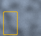The black border in the left image looks as if it outlines the black region in the right image, which agrees with the prediction that only the transition region becomes darker.

Some Questions

The maximum value returned by noise(p) in the code is 1, and the initial value of weight is also 1. Therefore, abs(accum) can be greater than 1. This clearly makes no sense, because a ray cannot become brighter after hitting an object (other than a light source). I previously emailed the author of this blog about the question, but he said that he did not know either; perhaps values greater than 1 are simply rare because of probability.

I then looked at Ken Perlin’s 1985 SIGGRAPH paper^[3]. It contains neither a very rigorous description nor actual code, although the basic idea is clear. One thing I found strange is that the entire paper never says that the new noise algorithm is intended to improve value noise. It mainly focuses on the fact that the effect of Perlin noise is unaffected by various spatial transformations (did he invent a noise algorithm independent of spatial transformations and improve value noise along the way? That would be rather absurd):

Noise()
In order to get the most out of the PSE and the solid texture approach we have provided some primitive stochastic functions with which to bootstrap visual complexity. We now introduce the most fundamental of these. Noise() is a scalar valued function which takes a three dimensional vector as its argument. It has the following properties :

Statistical invariance under rotation (no matter how we rotate its domain, it has the same statistical character)

A narrow bandpass limit in frequency (its has no visible features larger or smaller than within a certain narrow size range)

Appendix. Turbulence
A suitable procedure for the simulation of turbulence using the Noise() signal is :
1
2
3
4
5
6
7
function turbulence(p)
  t = 0
  scale = 1
  while (scale > pixelsize)
      t += abs(Noise(p / scale) * scale)
      scale /= 2
  return t

The turbulence pseudocode is basically no different from the version in the book. For the Noise() function, however, Perlin only says that it takes the position of a point and returns a scalar, without specifying the scalar’s range, so the issue remains rather puzzling.

Nevertheless, a sentence later in the paper still makes it seem that he intended to return a value in the $[0, 1]$ range (he mentions using a color such as $[1, 1, 1]$ ):

By evaluating Noise() at visible surface points of simulated objects we may create a simple “random” surface texture (figure Spotted.Donut) :
color = white * Noise(point)

This question troubled me for quite a long time. If you know the correct explanation, you are welcome to leave it in the comments. I also plan to ask about it on Stack Overflow after a while; if I get an answer, I will update this blog post.

Instance Transformations

Rotation Matrices

Formula Derivation

When I first saw the following formulas in the book, I was rather confused:

$x^\prime = \cos(\theta) - \sin(\theta) \cdot y \\ y^\prime = \sin(\theta) + \cos(\theta) \cdot y$

After searching online, I found that this is actually a rotation matrix. The formula is derived as follows (the preceding formula describes rotation around the z-axis, which we can understand simply as a rotation matrix in a two-dimensional plane)

$x = r\cos\phi \\ y = r\sin\phi$

Add $\theta$ to the original angle:

$x^\prime = r\cos(\phi + \theta) \\ y^\prime = r\sin(\phi + \theta)$

Use the following two angle-sum formulas:

$\cos(\phi + \theta) = \cos\phi\cos\theta - \sin\phi\sin\theta \\ \sin(\phi + \theta) = \sin\phi\cos\theta + \cos\phi\sin\theta$

Substitute the polar-coordinate form of $(x^\prime, y^\prime)$ :

$\begin{align*} x^\prime &= r(\cos\phi\cos\theta - \sin\phi\sin\theta) \\ x^\prime &= (r\cos\phi)\cos\theta - (r\sin\phi)\sin\theta \\ x^\prime &= x\cos\theta - y\sin\theta \end{align*}$

$\begin{align*} y^\prime &= r(\sin\phi\cos\theta + \cos\phi\sin\theta) \\ y^\prime &= r(\sin\phi)\cos\theta + r(\cos\phi)\sin\theta \\ y^\prime &= y\cos\theta + x\sin\theta \\ &= x\sin\theta + y\cos\theta \end{align*}$

Some Explanations

Rotation around the $x$ -axis is basically no different from this, but rotation around the $y$ -axis is rather puzzling. Rotations around the other two axes both have the form $\cos - \sin$ , $\sin + \cos$ , but for rotation around the $y$ -axis alone, the form becomes $\cos + \sin$ and $-\sin + \cos$ .

Because the sign of $\sin$ changes in a rotation around $y$ , it is obvious that we are actually rotating not by $\theta$ but by $-\theta$ . This is because the rotation direction we want is “different” from the rotation direction in a right-handed coordinate system.

That statement is vague, so we can proceed one step at a time and first determine the direction in which we want to rotate:

           y+
           |
           | 
           |
x- ------- z --------- x+
           |
           |
           |
           y-

This diagram shows a right-handed coordinate system viewed along the $z$ -axis. Note that the positive direction of the $z$ -axis points toward the observer. Clearly, if I say that I want to rotate something by $90^\circ$ around the $z$ -axis, I expect it to move from the positive $x$ direction to the positive $y$ direction. Equivalently, $y+ \to x-$ , $x- \to y-$ , and $y- \to x+$ ; in short, the rotation is counterclockwise.

Now consider rotation around the $x$ -axis:

           y+
           |
           | 
           |
z+ ------- x --------- z-
           |
           |
           |
           y-

Again, the $x$ -axis points toward the observer, so the rotation is counterclockwise, from $y+$ to $z+$ .

Now include the formulas and see whether they agree with our expectation—that is, a rotation from $y+$ to $z+$ .

Suppose the current point is $(x, y, z) = (0, 1, 0)$ (that is, it lies on $y+$ ). After a rotation of $90^\circ$ , $(x^\prime, y^\prime, z^\prime)$ should lie on $z+$ , namely at $(0, 0, 1)$ .

First consider the formula for $y^\prime$ :

$\begin{align*} y^\prime &= \cos \theta \cdot y - \sin\theta \cdot z \\ &= \cos(90) \cdot 1 - \sin(90) \cdot 0 \\ &= 0 - 0 = 0 \end{align*}$

Next, consider $z^\prime$ :

$\begin{align*} z^\prime &= \sin \theta \cdot x + \cos \theta \cdot z \\ &= \sin(90) \cdot 1 + \cos(90) \cdot z \\ &= 1 + 0 = 1 \end{align*}$

It appears to be correct.

Now consider rotation around the $y$ -axis:

           z-
           |
           | 
           |
x- ------- y --------- x+
           |
           |
           |
           z+

We find that if we still rotate counterclockwise by $90^\circ$ and start on $x+$ , the point should move to $z-$ . If we continue using the formula for the other two axes, however, it moves to $z+$ instead, as follows:

$\begin{align*} z^\prime &= \sin \theta \cdot x + \cos \theta \cdot z \\ &= \cos(90) \cdot 0 - \sin(90) \cdot -1 \\ &= 0 - (1 \cdot -1) = 1 \end{align*}$

Sure enough, changing the sign of $\sin$ in the formula solves the problem.

What is special about rotation around $y$ ? Consider an example. For rotations around the other two axes, if the direction of the rotation angle is counterclockwise and the rotation goes from the lower-numbered axis to the higher-numbered axis (such as $x \to y$ or $y \to z$ ), the directions of those two axes are the same ( $x+ \to y+$ and $x- \to y-$ ).

For rotation around the $y$ -axis, if we rotate counterclockwise from the lower-numbered axis to the higher-numbered axis, the directions of those two axes differ ( $x+ \to z-$ and $x- \to z+$ ).

After all, trigonometric functions were originally designed for the Cartesian plane (the xy-plane). When they are applied to a plane with different signs, some adjustment is inevitably required.

You may now wonder whether changing to a left-handed coordinate system would solve the problem. The answer is both yes and no. Rotation around the $y$ -axis would indeed no longer require changing the sign of $\sin$ , but rotation around the $z$ -axis would require it. Reversing the direction of the $z$ -axis is equivalent to viewing the previous xy-plane from the opposite side, so a counterclockwise rotation from $x$ to $y$ becomes $-x \to +y$ or $+x \to -y$ .