How PWM Frequency Affects Electromagnet Current and Power Consumption

The content below was generated entirely by machine translation. Please verify its accuracy. If anything is unclear, consult the Chinese source version.

Problem Overview

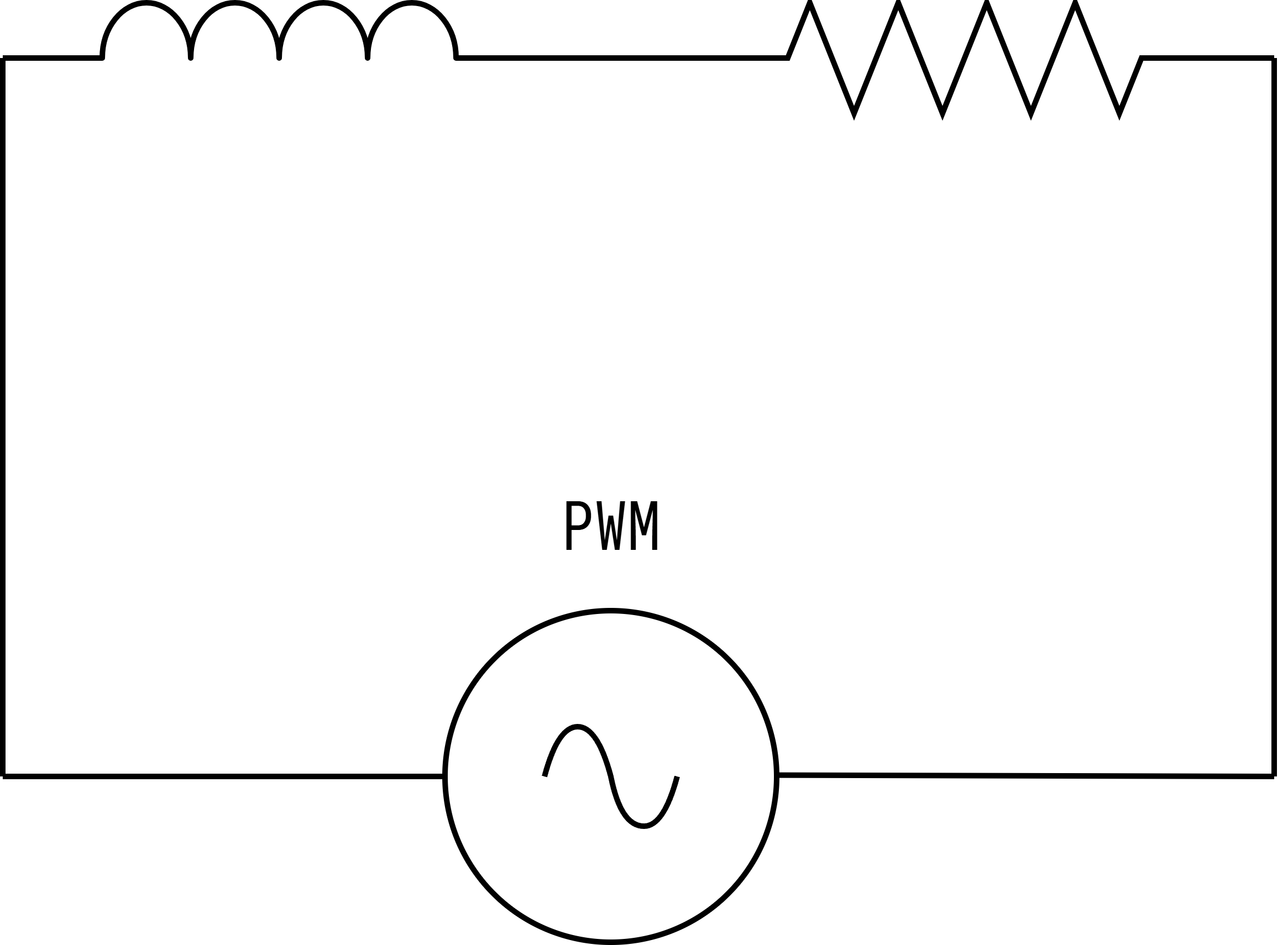
I have recently been working on a project involving PWM control of an electromagnet, and I was surprised to find that PWM at different frequencies seemed to produce different power consumption at the same duty cycle. I therefore did some simple calculations and analysis and have put the results here.

Here, the resistance R mainly comes from the resistance of the enamelled wire itself; the inductance L describes the relationship between the magnetic flux linkage in the coil and the current. When the current changes, the coil produces an induced electromotive force and, according to Lenz’s law, opposes changes in the current and magnetic flux.

Current Under Constant Voltage

Because PWM can be regarded as a periodic piecewise function, we can first consider the simplest case under constant voltage and then consider the piecewise function of PWM. For $V(t) = V_0$, the differential equation of the LR system is:

$$L \frac{di}{dt} + Ri = V_0$$

For the homogeneous solution, write the corresponding characteristic equation:

$$\begin{aligned} L r + R &= 0 \\ r &= - \frac{R}{L} \end{aligned}$$

Therefore, the homogeneous solution is:

$$i_h(t) = C e^{-\frac{R}{L} t}$$

The time constant can be defined as:

$$\tau = \frac{L}{R}$$

The homogeneous solution can then be written as:

$$i_h(t) = C e^{-\frac{t}{\tau}}$$

Because the input voltage is constant, we can guess that the particular solution is a constant $i_p(t) = A$. Substituting it into the differential equation gives:

$$RA = V_0 \quad \text{because} \space \frac{di_p}{dt} = 0$$

Therefore,

$$i_p = \frac{V_0}{R}$$

Combining the homogeneous and particular solutions gives the general solution:

$$i(t) = C e^{-\frac{t}{\tau}} + \frac{V_0}{R}$$

Next, determine the constant $C$ from the initial condition. Assume that the initial current is $i(0) = i_0$. Substitution gives:

$$\begin{aligned} i_0 &= C + \frac{V_0}{R} \\ C &= i_0 - \frac{V_0}{R} \end{aligned}$$

The final result is:

$$i(t) = \frac{V_0}{R} + \left(i_0 - \frac{V_0}{R}\right) e^{-\frac{t}{\tau}}$$

Drag the sliders below to observe how the time constant $\tau$, initial current $i_0$, and DC steady-state current $i_f\,(V_0/R)$ affect the current response. The part of the graph where $t<0$ remains at the initial current, and the response begins at $t=0$.

Loading chart...

The first term is the DC steady-state current, while the second is the continuously decaying transient current.

Current Under PWM

For a PWM signal with period $T$ and duty cycle $D$, its voltage can be expressed as:

$$V(t) = \begin{cases} V_0 & 0 \leq t < DT \\ 0 & DT \leq t < T \end{cases}$$

The graph below shows the periodically repeating PWM voltage. The duty cycle $D$, period $T$, and high-level voltage $V_0$ can be adjusted.

Loading chart...

Cycle Peak and Valley Currents

Let the DC steady-state current be $i_f = V_0/R$, and assume that the initial current is $i_0 = 0$. Then, at the first transition from the high level to the low level, the current is:

$$\begin{aligned} i_{\text{max1}} &= i_f + (0 - i_f)e^{-\frac{DT}{\tau}}\\ & = i_f(1 - e^{-\frac{DT}{\tau}}) \end{aligned}$$

Let $E = 1 - D$. Then, at the first transition from the low level to the high level, the current is:

$$\begin{aligned} i_\text{min1} &= i_{\text{max1}} e^{-\frac{ET}{\tau}} \\ &= i_f\left(1 - e^{-\frac{DT}{\tau}}\right) e^{-\frac{ET}{\tau}} \end{aligned}$$

We can observe that the current in each state can be calculated from the current in the preceding state and the time constant $\tau$. Therefore, the following recurrence relations can be written:

$$\begin{aligned} i_\text{max(n)} &= i_f + (i_\text{min(n-1)} - i_f)e^{-\frac{DT}{\tau}} \\ i_\text{min(n)} &= i_\text{max(n)} e^{-\frac{ET}{\tau}} \end{aligned}$$

To make the pattern easier to observe, continue by listing several transitions. The following is the second transition from the high level to the low level:

$$\begin{aligned} i_\text{max2} &= i_f + (i_\text{min1} - i_f)e^{-\frac{DT}{\tau}} \\ &= i_f + \left(i_f e^{-\frac{ET}{\tau}} - i_f e^{-\frac{DT}{\tau}}e^{-\frac{ET}{\tau}} - i_f\right)e^{-\frac{DT}{\tau}} \\ &= i_f\left(1 + e^{-\frac{T}{\tau}} - e^{-(D + 1)\frac{T}{\tau}} - e^{-\frac{DT}{\tau}}\right) \\ &= i_f\left(1 - e^{-\frac{DT}{\tau}} + e^{-\frac{T}{\tau}} - e^{-(D + 1)\frac{T}{\tau}}\right) \\ \end{aligned}$$

The second transition from the low level to the high level is:

$$\begin{aligned} i_\text{min2} &= i_\text{max2} e^{-\frac{ET}{\tau}} \\ &= i_f\left(e^{-\frac{ET}{\tau}} - e^{-\frac{T}{\tau}} + e^{-(E+1)\frac{T}{\tau}} - e^{-\frac{2T}{\tau}}\right) \end{aligned}$$

The third transition from the high level to the low level is:

$$\begin{aligned} i_\text{max3} &= i_f + (i_\text{min2} - i_f)e^{-\frac{DT}{\tau}} \\ &= i_f\left(1 + e^{-\frac{T}{\tau}} - e^{-(D+1)\frac{T}{\tau}} + e^{-\frac{2T}{\tau}} - e^{-(D+2)\frac{T}{\tau}} - e^{-\frac{DT}{\tau}}\right) \\ &= i_f\left(\textcolor{red}{1} - \textcolor{blue}{e^{-\frac{DT}{\tau}}} + \textcolor{red}{e^{-\frac{T}{\tau}}} - \textcolor{blue}{e^{-(D + 1)\frac{T}{\tau}}} + \textcolor{red}{e^{-\frac{2T}{\tau}}} - \textcolor{blue}{e^{-(D + 2)\frac{T}{\tau}}}\right) \end{aligned}$$

Notice that the odd-numbered terms (red) and even-numbered terms (blue) in the equation above can each be generalized as a geometric sequence. Both have the common ratio $e^{-\frac{T}{\tau}}$, but their first terms differ. Let $k = \frac{T}{\tau}$; the general formula can be written as:

$$\begin{aligned} i_\text{max(n)} &= i_f\left(\sum_{j=0}^{n-1}e^{-jk} - \sum_{j=0}^{n-1}e^{-(D+j)k} \right)\\ &= i_f\left(\sum_{j=0}^{n-1} e^{-jk} - e^{-Dk}\sum_{j=0}^{n-1} e^{-jk} \right)\\ &= i_f\left( 1-e^{-Dk} \right)\sum_{j=0}^{n-1} e^{-jk} \\ \end{aligned}$$

After letting $n\to\infty$, use the infinite geometric series sum formula $\frac{a}{1-r}$, where the first term is $a=i_f(1-e^{-Dk})$ and the common ratio is $r=e^{-k}$. This gives:

$$\lim_{n \to \infty} i_\text{max(n)} = i_\text{max} = i_f\frac{1 - e^{-Dk}}{1 - e^{-k}}$$

Note that this series converges only when $|e^{-k}| < 1$, that is, $-k < 0 \implies k > 0$. Because $T, \tau > 0$, this condition is clearly always satisfied.

According to the recurrence formula above, the current at each transition from the low level to the high level is:

$$\begin{aligned} i_\text{min} &= i_\text{max} e^{-\frac{ET}{\tau}} \\ &= i_f \frac{e^{-Ek}\left(1 - e^{-Dk}\right)}{1 - e^{-k}} \\ &= i_f \frac{e^{-Ek} - e^{-k}}{1 - e^{-k}} \\ &= i_f \frac{e^{-(1-D)k} - e^{-k}}{1 - e^{-k}} \quad \text{divide the numerator and denominator by} \space e^{-k} \\ &= i_f \frac{e^{Dk} - 1}{e^{k} - 1} \end{aligned}$$

Next, let the frequency be $f=1/T$ and observe how the cycle peak current $i_\text{max}$ and cycle valley current $i_\text{min}$ vary with PWM frequency after the system has entered the periodic steady state. The horizontal axis uses a logarithmic scale, and the duty cycle $D$, time constant $\tau$, and DC steady-state current $i_f\,(V_0/R)$ can be adjusted.

The buttons inside the graph can be used to switch between logarithmic and linear coordinates.

Loading chart...

We can observe that, as the frequency increases, the current fluctuation amplitude decreases and approaches the product of the DC steady-state current and the duty cycle, $i_f D$. Taking the limits of the cycle peak current $i_\text{max}$ and the cycle valley current $i_\text{min}$ separately gives the following. Because both expressions are of the form $\frac{0}{0}$ as $k\to 0$, differentiate the numerator and denominator separately with respect to $k$ and apply L’Hôpital’s rule:

$$\begin{aligned} f \to \infty &\implies k \to 0,\\ \lim_{k \to 0} i_\text{max} &= i_f\lim_{k \to 0}\frac{1-e^{-Dk}}{1-e^{-k}}\\ &= i_f\lim_{k \to 0}\frac{D e^{-Dk}}{e^{-k}} \\ &= i_f D \\ \end{aligned}$$

$$\begin{aligned} \lim_{k \to 0} i_\text{min} &= i_f\lim_{k \to 0}\frac{e^{Dk}-1}{e^k-1}\\ &= i_f\lim_{k \to 0}\frac{De^{Dk}}{e^{k}}\\ &= i_f D \end{aligned}$$

The calculated result agrees with the graph above.

Period-Average Current

The preceding calculations obtained the cycle peak current $i_\text{max}$ and cycle valley current $i_\text{min}$. We can therefore calculate the relationship between the period-average current $\overline{i}$ and the duty cycle $D$.

The average current over one period is the sum of the current integrals over the on and off stages divided by the period $T$:

$$\overline{i} = \frac{1}{T} \left[ \int_0^{DT} i_\text{on}(t)\,dt + \int_0^{(1-D)T} i_\text{off}(t)\,dt \right].$$

The currents during the on and off stages are, respectively:

$$\begin{aligned} i_\text{on}(t) &=i_f+(i_\text{min}-i_f)e^{-t/\tau},\\ i_\text{off}(t) &=i_\text{max}e^{-t/\tau}. \end{aligned}$$

Therefore:

$$\begin{aligned} \overline{i} &= \frac{1}{T} \left[ \int_0^{DT} \left( i_f+(i_\text{min}-i_f)e^{-t/\tau} \right)dt + \int_0^{(1-D)T} i_\text{max}e^{-t/\tau}dt \right]\\ &= \frac{1}{T} \left[ i_fDT + \tau(i_\text{min}-i_f)(1-e^{-Dk}) + \tau i_\text{max}(1-e^{-(1-D)k}) \right]. \end{aligned}$$

According to the endpoint relationship of the on stage:

$$i_\text{max} = i_f+(i_\text{min}-i_f)e^{-Dk},$$

therefore:

$$\begin{aligned} (i_\text{min}-i_f)(1-e^{-Dk}) &=i_\text{min}-\left[i_f+(i_\text{min}-i_f)e^{-Dk}\right]\\ &=i_\text{min}-i_\text{max}. \end{aligned}$$

For the off stage, we also have:

$$i_\text{min}=i_\text{max}e^{-(1-D)k},$$

therefore:

$$i_\text{max}(1-e^{-(1-D)k}) =i_\text{max}-i_\text{min}.$$

The two exponential integral terms cancel exactly:

$$(i_\text{min}-i_\text{max})+(i_\text{max}-i_\text{min})=0.$$

Therefore:

$$\begin{aligned} \overline{i} &=\frac{i_fDT}{T}\\ &=i_fD. \end{aligned}$$

Thus, the period-average current is independent of the PWM frequency and equals the product of the DC steady-state current $i_f$ and the duty cycle $D$.

For an ideal energized solenoid, the magnetic field strength satisfies $H=nI$, while the magnetic flux density satisfies $B=\mu H=\mu nI$, where $\mu$ is the permeability and $n$ is the number of turns per unit length. The relationship above therefore shows that, under this ideal model, the electromagnet’s average magnetic field strength is independent of frequency and varies linearly with the duty cycle.

Power Under PWM

For an LR system, the average power of the inductor is zero, as can be shown by the following process.

The inductor voltage satisfies:

$$V_L(t) = L \frac{di}{dt}$$

Substituting this into $P = VI$ gives:

$$P_L(t) = L i \frac{di}{dt}$$

For a PWM signal with period $T$, the average power of the inductor is:

$$\begin{aligned} \overline{P_L} &= \frac{1}{T}\int_{t_0}^{t_0 + T} P_L(t) dt \\ &= \frac{1}{T}\int_{t_0}^{t_0 + T} L i \frac{di}{dt} dt \\ &= \left. \frac{1}{2T} L i^2 \right|_{t_0}^{t_0 + T} \\ \end{aligned}$$

Because the current $i(t)$ is periodic over one period, $i^2(t)$ is also periodic, and its values at the beginning and end of the period are equal. Therefore:

$$i^2(t_0+T)-i^2(t_0)=0.$$

Thus, the boundary term above is zero, and the average power of the inductor over one period is also zero.

Therefore, in the period-average sense, only the power dissipated by the resistor remains in the entire system:

$$P_R(t) = i^2(t)R$$

Now consider the average input power $\overline{P}$ over one complete period after the system has entered the periodic steady state. Divide the PWM period into the off and on stages. During the off stage, $V=0$, so the input power from the source, $V(t)i(t)$, is zero; however, the resistor continues to dissipate power at $i^2(t)R$, with the energy released by the inductor. During the on stage, the following relationship is obtained:

$$\begin{aligned} \overline{P} &= \frac{1}{T} \int_{t_0}^{t_0 + T} V(t)i(t) dt\\ &= \frac{V_0}{T} \int_0^{DT} i_\text{on}(t) dt \\ \end{aligned}$$

During the on stage, the current can be understood as rising gradually from the cycle valley current $i_\text{min}$ to the cycle peak current $i_\text{max}$ with the time constant $\tau$. Therefore, we can write:

$$\begin{aligned} \overline{P} &= \frac{V_0}{T} \int_0^{DT}\left[i_f + (i_\text{min} - i_f)e^\frac{-t}{\tau} \right]dt \end{aligned}$$

Because:

$$\int_0^{DT} e^\frac{-t}{\tau} dt = \tau \left(1 - e^{-\frac{DT}{\tau}} \right)$$

substituting the integral result into the equation above gives:

$$\begin{aligned} \overline{P} &= \frac{V_0}{T} \left[ i_fDT + \tau(i_\text{min}-i_f) \left(1-e^{-\frac{DT}{\tau}}\right) \right] \\ &= V_0i_fD + V_0\frac{\tau}{T}(i_\text{min}-i_f) \left(1-e^{-Dk}\right) \end{aligned}$$

Also, because we have already defined:

$$k=\frac{T}{\tau}, \qquad E=1-D,$$

we have:

$$\frac{\tau}{T}=\frac{1}{k}.$$

Next, simplify $i_\text{min}-i_f$. According to the expression for $i_\text{min}$ obtained above:

$$i_\text{min} = i_f\frac{e^{Dk}-1}{e^k-1},$$

we obtain:

$$\begin{aligned} i_\text{min}-i_f &= i_f \left( \frac{e^{Dk}-1}{e^k-1}-1 \right) \\ &= i_f \frac{e^{Dk}-e^k}{e^k-1} \\ &= -i_f\frac{e^k-e^{Dk}}{e^k-1} \\ &= -i_f\frac{1-e^{-(1-D)k}}{1-e^{-k}} \\ &= -i_f\frac{1-e^{-Ek}}{1-e^{-k}}. \end{aligned}$$

Substitute this back into the expression for the average power:

$$\begin{aligned} \overline{P} &= V_0i_fD - V_0\frac{\tau}{T} i_f \frac{1-e^{-Ek}}{1-e^{-k}} \left(1-e^{-Dk}\right) \\ &= V_0i_f \left[ D - \frac{1}{k} \frac{ \left(1-e^{-Dk}\right) \left(1-e^{-Ek}\right) }{ 1-e^{-k} } \right]. \end{aligned}$$

Because:

$$i_f=\frac{V_0}{R},$$

define the DC power as $P_{\mathrm{ref}}=V_0i_f=\frac{V_0^2}{R}$. Therefore:

$$\overline{P} = P_{\mathrm{ref}} \left[ D - \frac{1}{k} \frac{ \left(1-e^{-Dk}\right) \left(1-e^{-Ek}\right) }{ 1-e^{-k} } \right]$$

Then substitute $E=1-D$:

$$\overline{P} = P_{\mathrm{ref}} \left[ D - \frac{1}{k} \frac{ \left(1-e^{-Dk}\right) \left(1-e^{-(1-D)k}\right) }{ 1-e^{-k} } \right]$$

Finally, use:

$$f=\frac{1}{T}, \qquad k=\frac{T}{\tau}=\frac{1}{f\tau}, \qquad \frac{1}{k}=f\tau,$$

to write the average power as a function of PWM frequency and duty cycle:

$$\overline{P}(f,D) = P_{\mathrm{ref}} \left[ D - f\tau \frac{ \left(1-e^{-\frac{D}{f\tau}}\right) \left(1-e^{-\frac{1-D}{f\tau}}\right) }{ 1-e^{-\frac{1}{f\tau}} } \right]$$

Here, $f\tau$ is a dimensionless quantity. The result obtained here is the average input power from the source over one period. Because the inductor’s average power is zero in the periodic steady state, it is also equal to the average power dissipated by the resistor over one period.

Chart Analysis

Below, we separately observe how the period-average power varies with the duty cycle $D$ and PWM frequency $f$. Here, $P_{\mathrm{ref}}=\frac{V_0^2}{R}$ is adjusted as a whole and represents the DC power.

Period-Average Power Versus Duty Cycle

The horizontal axis is the duty cycle $D$. The frequency $f$, time constant $\tau$, and DC power $P_{\mathrm{ref}}$ can be adjusted. The frequency slider uses logarithmic adjustment.

The graph also shows the linear reference $P_{\mathrm{ref}}D$ and quadratic reference $P_{\mathrm{ref}}D^2$ for comparing the trends at low and high frequencies.

Loading chart...

Period-Average Power Versus Frequency

The horizontal axis is the frequency $f$ and uses a logarithmic scale. The duty cycle $D$, time constant $\tau$, and DC power $P_{\mathrm{ref}}$ can be adjusted.

The button inside the graph can be used to switch to linear coordinates.

Loading chart...

Normalized Period-Average Power Contour Plot

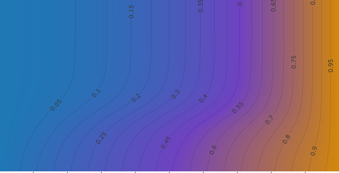
The contour plot presents the same function from a top-down view. Its horizontal axis is $D$, its vertical axis is $f\tau$, and both the colors and contour values represent $\overline P/P_{\mathrm{ref}}$.

Loading chart...

The three graphs above show that, as the frequency increases, the power approaches the quadratic reference $\overline{P}(D) = P_{\mathrm{ref}} D^2$, whereas at low frequencies the variation in power is closer to the linear reference $\overline{P}(D) = P_{\mathrm{ref}} D$. In other words, at the same duty cycle, because $\forall D \in [0, 1] \quad D^2 \le D$, the power consumption of high-frequency PWM is always lower than or equal to that of low-frequency PWM.

Note that in the “Period-Average Current” section, we have already concluded that the electromagnet’s average magnetic field strength is related to the duty cycle and independent of frequency. Combining this with the power analysis shows that using a higher PWM frequency to control an electromagnet is always more energy-efficient.

Understanding Through Variance

From the preceding discussion, the period-average power consumption $\overline{P}$ depends only on the period-average resistive power $\overline{i^2}R$, while the average power of the inductor is zero. Notice that $\overline{i^2}$ has a form similar to the variance formula:

$$\text{Var}(i) = \langle i^2\rangle - \langle i \rangle^2$$

Here, $\langle i \rangle$ represents the average value of $i$ over one period and has the same meaning as $\overline{i}$. Rearranging gives:

$$\langle i^2\rangle = \text{Var}(i) + \langle i \rangle^2$$

Substituting this back into the average-power formula gives:

$$\overline{P} = \langle i \rangle^2R + \text{Var}(i)R$$

From the “Period-Average Current” section, we know that $\langle i \rangle$ is independent of frequency. Variance measures the amplitude of current fluctuations. As the frequency increases, the current ripple decreases, the current waveform approaches the constant value $i_fD$, and the power consumption gradually decreases.